Statistical process control (SPC) is defined as the use of statistical techniques to control a process or production method. SPC tools and procedures can help you monitor process behavior, discover issues in internal systems, and find solutions for production issues.
Though SPC has effectively been used in western industries since 1980, it was started during the twenties in America. Walter A Shewhart, developed the control chart and the concept that a process could be under statistical control in 1924 at Bell Telephone Laboratories, USA. The SPC concepts are included in the management philosophy by Dr. W.E. Deming just before World War II. However, SPC became famous after Japanese industries implement the concepts and compete with western industries.
Why use Statistical Process Control
Today companies are facing increasing competition and also operational costs, including raw materials continuously increasing. So for the organizations, it is beneficial if they have control over their operation.
Organizations must make an effort for continuous improvement in quality, efficiency, and cost reduction. Many organizations still follow inspection after production for quality-related issues.
SPC helps companies to move towards prevention-based quality control instead of detection-based quality controls. By monitoring SPC graphs, organizations can easily predict the behavior of the process.
Statistical Process Control Benefits
- Reduce scrap and rework
- Increase productivity
- Improve overall quality
- Match process capability to product requirement
- Continuously monitor the process to maintain control
- Provide data to support decision making
- Streamline the process
- Increase in product reliability
- Opportunity for company-wide improvements
Statistical Process Control Objective
SPC focuses on optimizing continuous improvement by using statistical tools to analyze data, make inferences about process behavior, and then make appropriate decisions.
The basic assumption of SPC is that all processes are subject to variation. Variation measures how data are spread around the central tendency. Moreover, variation may be classified as one of two types, random or chance cause variation and assignable cause variation.
Common Cause: A cause of variation in the process is due to chance, but is not assignable to any factor. It is the variation that is inherent in the process. The process under the influence of a common cause will always be stable and predictable.
Assignable Cause: It is also known as “special cause”. The variation in a process that is not due to chance therefore can be identified and eliminated. The process under influence of a special cause will not be stable and predictable.
How to Perform SPC
- Identify the processes: Identify the key process that impacts the output of the product or the process that is very critical to the customer. For example, plate thickness impacts the product’s performance in a manufacturing company, then consider the plate manufacturing process.
- Determine measurable attributes of the process: Identify the attributes that need to measure during the production. From the above example, consider the plate thickness as a measurable attribute.
- Determine the measurement method and also perform Gage R&R: Create a measurement method work instructions or procedure including the measuring instrument. For example, consider thickness gage to measure the thickness and create an appropriate measuring procedure. Perform Gage Repeatability and Reproducibility (Gage R & R) to define the amount of variation in the measurement data due to the measurement system.
- Develop a subgroup strategy and sampling plan: Determine the subgroup size based on the product’s criticality and determine the sampling size and frequency. For example, collect 20 sets of plate thicknesses in a time sequence with a subgroup size of 4.
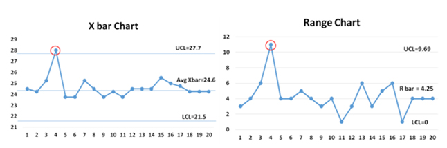
- Collect the data and plot the SPC chart: Collect the data as per sample size and select an appropriate SPC chart based on data type (Continuous or Discrete) and also subgroup size. For Example, for plate thicknesses with a subgroup size of 4, select Xbar -R chart.
- Describe natural variation of attributes: Calculate the control limits. From the above example, calculate the upper control limit (UCL) and lower control limit (LCL) for both Xbar Range.
- Monitor process variation: Interpret the control chart and check whether any point is out of control and the pattern. Example: check the Xbar R chart If the process is not in control, then identify the assignable cause(s) and address the issue. This is an ongoing process to monitor the process variation.